
The recipe says 160 C. But what does that mean to YOUR oven? Do you have to hover over it, tense and alert like a Marine in a flame-lit chamber left only with his fists and 3 imps bearing down?
If you’ve never played DOOM, you can find an abundance of sources by typing ‘play doom online’ into Google but for goodness’ sake find SOMETHING better to do than standing over your oven micro-managing the settings! Get yourself one of these beauties:
or you can really geek out and buy a wireless thermometer. Now scroll down to find out how to go into oven calibration overdrive armed with a bit of R and a genuine love of data nerd-dom. Or if the R and nerdville-ness of it all leaves you as cold as your oven leaves the centre of your dinner, you can send us your oven setting vs actual temperature numbers and we’ll send you back your personalised calibration table.
Here’s how our great oven caper went down.
When we dial our oven to 160 C, a 45 minute cake will be burnt on top and raw inside in under 25 minutes. Charcoaly and gooey!
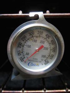
So we bought the elegant and attractive oven thermometer pictured above for approx. $9.95,
Now …
Stand back! I’m going to science!
Before you can science you need a question
The question I want answered:
“If the recipe says 170 C, what temperature do I set the dial to? What about 150 C? What then?”
We’re going to need a calibration line to answer that!
Finding our oven calibration line in R
What I did: I ran the oven at a few temperature settings, letting it steady out each time, and wrote down what the oven thermometer said.
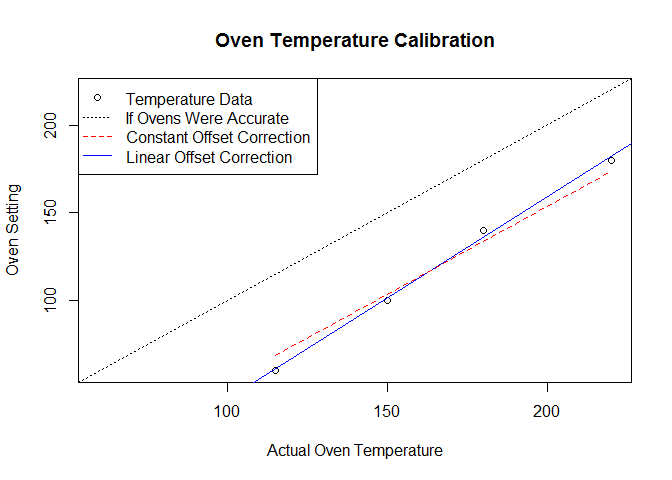
First, the data, and a plot. “x” is the actual oven temperature, “y” is the dial setting
# x - the oven temperature.
# y - the temperature setting.
x <- c(115,150,180,220)
y <- c(60,100,140,180)

plotlims <- range(c(x,y))

ovenPlot <- function(xval=x,yval=y,xl=plotlims, yl=plotlims) {
  plot(yval ~ xval, xlim=xl, ylim=yl,
       main="Oven Temperature Calibration",
       ylab="Oven Setting",
       xlab="Actual Oven Temperature")
  abline(0,1, lty=3)
}

ovenPlot()
legend(
  "topleft",
  legend=c("Temperature Data",
           "If Ovens Were Accurate"),
  lty=c(NA,3),
  pch=c(1,NA),
  col=c("black","black")
)
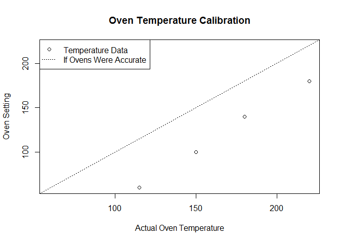
Ok, we’re off by a lot. So is it a constant offset? Like, “just subtract 50 degrees”? or does the offset change significantly with temperature?
Re-plot that, just as temperature difference.
plot(I(x-y) ~ x,
     main="Oven Thermostat Error",
     ylab="Error (Actual Temp minus Setting)",
     xlab="Actual Oven Temperature"
     )

Zooming in on the errors like this lets us see things that were less obvious in the previous plot. Even taking into account some normal temperature fluctuation, we can clearly see the oven runs too hot. How much it’s too hot decreases with temperature setting, but a 40+ degree error is a bit extreme. (The measurement at 180 C was a bit rushed, so I’m not surprised it’s not on the line).
Let’s try a constant offset by taking a kind of average of these points, and see how that looks.
lm.const <- lm(I(y - x) ~ 1)
summary(lm.const)
##
## Call:
## lm(formula = I(y - x) ~ 1)
##
## Residuals:
## 1 2 3 4
## -8.75 -3.75 6.25 6.25
##
## Coefficients:
## Estimate Std. Error t value Pr(>|t|)
## (Intercept) -46.25 3.75 -12.33 0.00115 **
## ---
## Signif. codes: 0 '***' 0.001 '**' 0.01 '*' 0.05 '.' 0.1 ' ' 1
##
## Residual standard error: 7.5 on 3 degrees of freedomovenPlot()
lines(x=x,y=(fitted(lm.const)+x),lty=2, col="red")
legend(
"topleft",
legend=c("Temperature Data",
"If Ovens Were Accurate",
"Constant Offset Correction"),
lty=c(NA,3,2),
pch=c(1,NA,NA),
col=c("black","black","red")
)
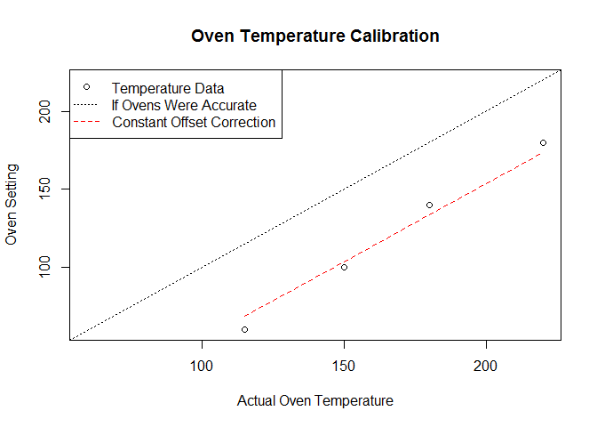
Seems ok. The constant is -46.25. So “Just subtract 45 from the recipe” seems like a pretty easy instruction to follow.
Let’s look at the correction error a bit more closely. This is the error between what the ‘just subtract 45deg’ correction says we should do to get temperature “x” and what temperature we actually get.
plot(resid(lm.const) ~ x,
     main="Constant Offset Correction",
     ylab="Correction Error",
     xlab="Actual Oven Temperature")
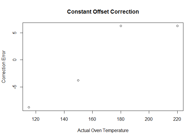
The correction errors (or “residuals”) have much the same shape as the first error plot, flipped upside-down. The scale is much smaller, which is good. My oven being 5 to 10 degrees off, I can live with.
But there’s still a pattern in the residuals, and that makes me want to try a little harder. Let’s see whether we can remove that pattern in the correction error. For fun, try a linear model.
Of course, fitting a two-parameter model to four data points is usually a silly choice. It often results in over-fitting, and when you do it for larger problems you can pretty much guarantee that cases outside the original “training” dataset won’t fit the model. In this case, our data covers our whole operating range, there’s every reason to believe that points between our data will follow the trend, and the consequences of being wrong are tiny. And this is fun.
My wife is fascinated by me. [Isn’t it your night to cook? -ed]
lm1 <- lm(y ~ x)
summary(lm1)
##
## Call:
## lm(formula = y ~ x)
##
## Residuals:
## 1 2 3 4
## -0.7539 -1.2147 4.1047 -2.1361
##
## Coefficients:
## Estimate Std. Error t value Pr(>|t|)
## (Intercept) -72.18848 7.56563 -9.542 0.01081 *
## x 1.15602 0.04433 26.080 0.00147 **
## ---
## Signif. codes: 0 '***' 0.001 '**' 0.01 '*' 0.05 '.' 0.1 ' ' 1
##
## Residual standard error: 3.425 on 2 degrees of freedom
## Multiple R-squared: 0.9971, Adjusted R-squared: 0.9956
## F-statistic: 680.1 on 1 and 2 DF, p-value: 0.001467ovenPlot()
abline(lm1, col="blue")
lines(x=x, y=x+fitted(lm.const),lty=2, col="red")
legend(
"topleft",
legend=c("Temperature Data",
"If Ovens Were Accurate",
"Constant Offset Correction",
"Linear Offset Correction"),
lty=c(NA,3,2,1),
pch=c(1,NA,NA,NA),
col=c("black","black","red","blue")
)
Let’s compare correction errors.
plot(resid(lm.const) ~ x,
     main="Correction Errors",
     ylab="Error",
     xlab="Actual Oven Temperature")

points(x,resid(lm1), pch=2)

legend(
  "topleft",
  legend=c("Constant Offset Correction",
           "Linear Offset Correction"),
  pch=c(1,2),
  col=c("black","black")
)
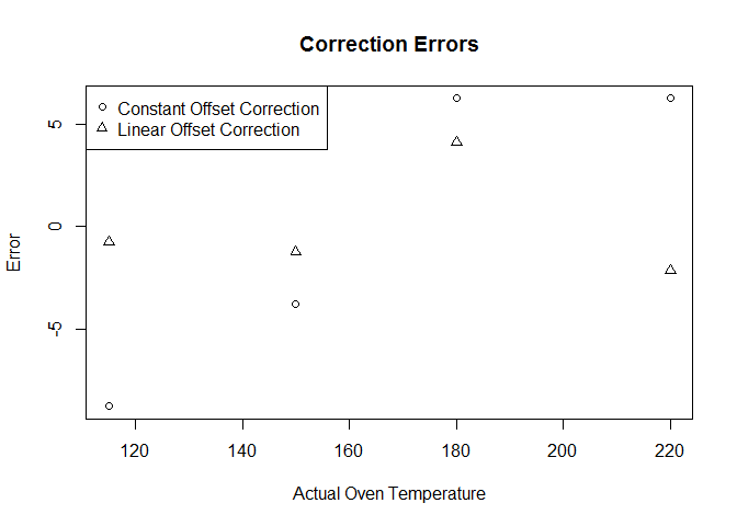
The second model offers two improvements:
- the errors are smaller (in fact, all are much closer to zero, even that dodgy 180degree reading)
- the errors look random-er
Graphically, both models look adequate. Both models show encouraging summary statistics. The linear offset model seems well-fitted, given the tiny data set.
At this point, which model is “the right one” depends on how fussy you are about being less than ten degrees off-target, and whether it’s worth your time and effort to reduce that.
This raises the usual question about “statistical significance” vs. “practical significance”.
Statistical significance means a difference we can reliably predict.
Practical significance means a statistically significant “difference that makes a difference”. Yes, it’s reliable and predictable. Do we care? That depends[3. When you read a study or report that might be “advertising disguised as science”, look for the words “statistically significant” without stating what the difference actually is. Advertisers love to impress people with science-y sounding terms like “statistical significance” to distract from the fact that it’s not a big enough difference to pay money for.].
Personally, I like the second model, and it gives me another five degrees of error correction. Also, we’d use the same correction method regardless of which model: tape a table of corrected values next to the oven (it can be difficult to reliably subtract 45 in one’s head when there are small children clutching one’s ankles and yelling about injustice and toys). So I’ll pick “method two”, even if it’s not strictly warranted.
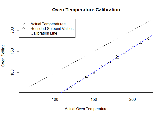
How to build a Calibration Table in R
Now, to build a calibration table:
x1 <- seq(120,220, by=10)
x1
## [1] 120 130 140 150 160 170 180 190 200 210 220y1 <- predict(lm1, newdata=data.frame(x=x1))
y1
##         1         2         3         4         5         6         7
##  66.53403  78.09424  89.65445 101.21466 112.77487 124.33508 135.89529
##         8         9        10        11
## 147.45550 159.01571 170.57592 182.13613
I’m not ever going to try set my oven to 112.77 C. We need to tidy that up. Let’s round everything to the nearest 5 degrees:
mround <- function(x,base){
  base*round(x/base)
}

y1r <- mround(y1,5)

ovenPlot()
abline(lm1, col="blue")
points(x1,y1r, pch=2)
legend("topleft",
       legend=c("Actual Temperatures",
                "Rounded Setpoint Values",
                "Calibration Line"),

       pch=c(1,2,NA),
       lty=c(0,0,1),
       col=c("black","black","blue")
)
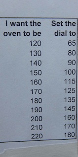
d1 <- data.frame("target" = x1, setting = y1r)
kable(d1, format="html",
      caption = "Proudly tape this next to oven.")
| target | setting |
|---|---|
| 120 | 65 |
| 130 | 80 |
| 140 | 90 |
| 150 | 100 |
| 160 | 115 |
| 170 | 125 |
| 180 | 135 |
| 190 | 145 |
| 200 | 160 |
| 210 | 170 |
| 220 | 180 |
And we did …
So now we can turn the dial and stop guessing, and cook things for the time specified in the recipe without having to hover and tweak things. Nice. Also, we can occasionally peek in and check on the oven temperature and see if it’s drifting even further off calibration.
Also, our oven thermostat probably needs fixing.[4. If your oven needs calibrating, feel free to contact us.]
[Also for clarity, when we use fan-force we do the normal -10 C from the recipe temperature to get our target temperature. And as you can see from the image of our home-made beef and beetroot sausage rolls, this calibration works perfectly for us. It is wonderful not to have to guess at temperature settings. And much cheaper than replacing or repairing the oven. -ed]
Leave A Comment